I recently finished an Undergraduate Research program run by the University of Sheffield mathematics department.
My subject was the highly abstract concept of “Mackey functors”. These are a niche but important part of many advanced mathematical concepts, including stable homotopy theory, and representation theory.
Their invention was motivated by trying to create a formal mathematical object which could find morphisms between different properties between a group and it’s subgroups. For instance, we may want to find a map between the order of a group’s subgroups. We may write a sketch to demonstrate what these mappings between subgroups should look like:

How do we formalise this into a concrete mathematical idea?
Category theory
In order to have any hope in defining such an object, we must explore a bit of category theory. But don’t worry, the initial definition is not actually too hard to understand!
A category  is comprised of two types of things, a collection of objects (
 ), and a collection of “morphisms” between these objects (
 ).
).
These are subject to two criteria, or axioms:
- For each object in
 in , there must exist an
  mophism
  such that
  for all compatible morphisms
  .
.  must be well-defined. That is, where we have morphisms in
  and
and  in
in  , we can find
  in
in  .
.
Some examples of categories include:
 – the category of sets. Contains all sets and all possible set mappings between these sets.
 – the category of abelian groups. All abelian groups and all homomorphisms between these abelian groups.
 – the category of groups. All groups and all homomorphisms between these groups.
 – the category of all small categories. Morphisms are “functors” (maps between categories).
 – the category of graphs. All possible graphs and all graph homomorphisms between them.
Definition by a function and axioms
One of the ways to define a Mackey functor is to use a function and then axiomatically enforce the existence of morphisms which go “up” subgroups and morphisms which go “down” subgroups. As the previously presented diagram suggests, we want our object to contain a morphisms to and from each pair of subgroups.
Consider a group  . A -Mackey functor
  is a function from the subgroups of to abelian groups in the
  of abelian groups, .
![\[\underline{M}: \{\text{subgroups of}~ G\} \to \mathbf{Ab}\]](https://henrytechblog.com/wp-content/ql-cache/quicklatex.com-9d09bdb28fe03752fedc2541a76f8673_l3.svg "Rendered by QuickLaTeX.com")
The category must contain the following morphisms…
![\[\text{Transfer} \colon ~~~ \text{tr}_{K}^{H} \colon \underline{M}(K) \to \underline{M}(H)\]](https://henrytechblog.com/wp-content/ql-cache/quicklatex.com-16a0cf051baba5f4809171a296b629a6_l3.svg "Rendered by QuickLaTeX.com")
![\[\text{Restriction}\colon ~~~ \text{res}_{K}^{H} \colon \underline{M}(H) \to \underline{M}(K)\]](https://henrytechblog.com/wp-content/ql-cache/quicklatex.com-bae910a46f417ed5754327bda516a870_l3.svg "Rendered by QuickLaTeX.com")
![\[\text{Conjugation}\colon ~~~ \text{c}_{g} \colon \underline{M}(H) \to \underline{M}(^{g}H)\]](https://henrytechblog.com/wp-content/ql-cache/quicklatex.com-9ee1386c96b7769343f1b0ba40442b06_l3.svg "Rendered by QuickLaTeX.com")
for all subgroups  of and all elements
  . The morphisms are subject to the following axioms:
![\[\begin{enumerate}\item $\text{tr}_{H}^{H}, \text{res}_{H}^{H}, \text{c}_{h} : \underline{M}(H) \to \underline{M}(H)$ are identity morphisms.\bigskip\item $\text{res}_{J}^{K}\text{res}_{K}^{H} = \text{res}_{J}^{H}$\bigskip\item $\text{tr}_{K}^{H}\text{tr}_{J}^{K} = \text{tr}_{J}^{H}$\bigskip\item $\text{c}_{g}\text{c}_{h} = \text{c}_{gh}$ for all $g, h \in G$.\bigskip\item $\text{res}_{^{g}K}^{^{g}H} \text{c}_g = \text{c}_{g} \text{res}_{K}^{H}$\bigskip\item $\text{tr}_{^{g}K}^{^{g}H} \text{c}_g = \text{c}_{g} \text{tr}_{K}^{H}$\bigskip\item $\text{res}_{J}^{H} \text{tr}_{K}^{H} = \sum_{x \in [J\setminus H / K]} \text{tr}_{J \cap ^{x}K}^{J} \text{c}_{x} \text{res}_{J^{x} \cap K}^{K}$ for all subgroups $J, K \le H$.\end{enumerate}\]](https://henrytechblog.com/wp-content/ql-cache/quicklatex.com-6205d9abe7b1aab23ba16de2728afa32_l3.svg "Rendered by QuickLaTeX.com")
Most of these rules are actually quite simple ideas. Most of them mathematicians are very familiar with, such as the idea that conjugation has to play well. For instance, if we reduce from  to
to  , then reduce again from to
  , we would expect that to be the same thing as reducing from to (this is what the second axiom is saying).
The axiom that doesn’t make sense is the notorious double coset formula – the last one. The story of why this axiom is included is quite interesting. It was originally included because it was a property that many examples of Mackey functor-like objects were exhibiting. It was then observed later on in a clever reformulation of the Mackey functor where it’s inclusion becomes undeniable.
Example: the constant Mackey functor
Let’s consider the constant  -Mackey functor.
We must define a mapping from each of the subgroups of to an abelian group. By definition, the constant Mackey functor assigns the same abelian group (we can call it ), to each of the subgroups.

We can then determine the restriction and transfer morphisms.
Restriction
The restriction morphism is  , so in this case, we simply define it as the inclusion map. As the domain of this function is a subset of the codomain, we can define a map which takes every element in the domain to the same element in the codomain. We can denote this as:
![\[\text{res}_{K}^{H} \colon \underline{M}(H) \xhookrightarrow{} \underline{M}(K)\]](https://henrytechblog.com/wp-content/ql-cache/quicklatex.com-60d97c7683859d47d15e6cb5a26f6dba_l3.svg "Rendered by QuickLaTeX.com")
Transfer / Conjugation
The transfer map is a bit more interesting. In the case of the constant Mackey functor, it happens that it is defined as so:
For a transfer  we define it as multiplying an element
  by the index of in (
 ). This is quite similar to what we were doing in the original example I gave of what a Mackey functor does – it’s revealed the change in size as we move up subgroups.

In this case conjugation is also just the identity morphism. All these groups are normal so conjugation does nothing to them.
You maybe wondering how we decided these functions are the transfer and restriction morphism. It all comes down to the axioms. We define this Mackey functor to take all subgroups to the same abelian group (hence “constant”), and then we look at the axioms. The restriction, transfer and conjugation we choose must satisfy the axioms, and the axiom that imposes the most limitation on what these can be is the double coset formula. By taking the double coset formula, we can cleverly choose subgroups so that the formula simplifies down and reveals some information about the morphism we are looking at. It is via this method that the correct function actually pops out.
Taking it further
This definition of a Mackey functor using a functor is nice enough, but you may have noticed that it’s a Mackey functor, not function. Let’s look at what a functor is
Functors
A functor is a mapping between categories. Given two categories and  , a functor creates an association from every object in , to a corresponding object
  in
in  , and similarly, for the morphisms in
  , it provides a morphism
  in
in  .
.
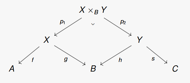
These maps are subject to maintaining proper composition. The functor must map composed morphisms in to the composition of the mapping of the individual morphisms, i.e.:  . This can be represented by the following commutative diagram:

Okay so with functors, we can map from a category to a category. So instead of mapping from the subgroups of to the category of abelian groups, and then axiomatically enforcing the existence of the morphisms we want, it would be nice to find a special category in which we can make a sensible assignment from each morphism in said category to restriction, transfer and conjugation.
That category turns out to be  . Using this object, we can create a full definition of a Mackey functor in just a few lines:
A Mackey functor is a functor
![\[\underline{F} \colon \text{Span}(\mathbf{FinGSet}) \to \mathbf{Ab}\]](https://henrytechblog.com/wp-content/ql-cache/quicklatex.com-c94e2a4f0e3ae95bd87c22fc3736fd7f_l3.svg "Rendered by QuickLaTeX.com")
which preserves products.
Thanks for reading!
 but there are even more definitions of factorials that mathematicians have invented.
 . It can be used to easily denote the product of the odd or even numbers less than or equal to n
![\[n!! =\left{\begin{matrix}n(n-2)(n-4) \cdots, \textrm{even n}\\n(n-2)(n-4)\cdots*1 , \textrm{odd n}\end{matrix}\right.\]](https://henrytechblog.com/wp-content/ql-cache/quicklatex.com-bdd250457ed5df78818f6e26d39f4d0f_l3.svg "Rendered by QuickLaTeX.com")
 ,
,![[1, 2, 3], [1, 3, 2], [2, 1, 3], [2, 3, 1], [3, 1, 2], [3, 2, 1]](https://henrytechblog.com/wp-content/ql-cache/quicklatex.com-e963560ec582c8e85b4357c1513fb513_l3.svg "Rendered by QuickLaTeX.com") .
. and
and 

 and is the product of primes less than and equal to n.


![\[n\$ = _{}^{n!}\textrm{n!}\]](https://henrytechblog.com/wp-content/ql-cache/quicklatex.com-109e46105f7518916dc873c80391bb43_l3.svg "Rendered by QuickLaTeX.com")
![\[4\$ = 24^{24\cdots^{24}}\]](https://henrytechblog.com/wp-content/ql-cache/quicklatex.com-08fd924480a2ac7b2ecbcf7230994130_l3.svg "Rendered by QuickLaTeX.com")
![\[n\$\]](https://henrytechblog.com/wp-content/ql-cache/quicklatex.com-89d9afab8b940460097ed9cb3fbce36e_l3.svg "Rendered by QuickLaTeX.com")
![\[4\$ = n^{n-1^{n-2}\cdots^{1}}\]](https://henrytechblog.com/wp-content/ql-cache/quicklatex.com-f8d9d87670b2f9fd357d150f321c023a_l3.svg "Rendered by QuickLaTeX.com")